

The Term Structure of Interest Rates and Macrofinancial Dynamics
August 17, 2017
In this speech, I will lay out a path to modeling macrofinancial dynamics using a recent approach that I have worked on, and illustrate the usefulness of this avenue with a term structure application.
We are not yet at a stage where we can say for sure that this generates the right magnitudes quantitatively, but I believe that my approach can point the way towards linking term structure dynamics and macrofinancial models in a novel fashion.
Let me start by inspecting four important aspects of interest rates:
- The level of the 10-year yield
- The term premium embedded in the 10-year yield
- Interest rate volatility as measured by the MOVE index
- The natural real rate r*
The term premium represents investors’ compensation for the risk that interest rates do not evolve as expected. The natural rate of interest is the real interest rate that prevails when monetary conditions are neutral.
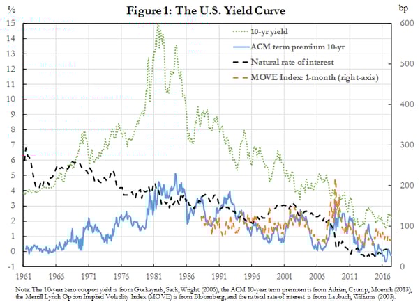
There are several salient features that warrant comment. First, the nominal rate rose from 4 percent in 1961 to a peak of 15 percent in 1982, before declining to below 2 percent in 2016. Some of that movement is closely associated with inflation. Second, the term premium rose from a level around 0 percent in 1961 to above 5 percent in 1985, and fell back to below 0 percent in 2016. The term premium spiked in 2008 during the global financial crisis. Third, the movements in volatility are tightly linked to the movements of the term premium. Fourth, the estimated level of the neutral rate exhibits a long term downward trend that is only tightly linked to the level of interest rates in recent years.
Any macrofinancial analysis of the term structure of interest rates takes a stance either explicitly or implicitly on the modeling of these important quantities—term premium, yield volatility, and the natural rate. Traditionally, macro models often assume that the term premium and interest rate volatility are constant. For example, that is the case in the standard New Keynesian (NK) model (Woodford, 2003 and Clarida, Gali, and Gertler, 1999), and those versions of the model that are often used in central banks (such as Christiano, Eichenbaum and Evans, 2005 or Smets and Wouters, 2007).[1] However, Figure 1 clearly shows that these quantities are time varying, and that the magnitude of variation in yields associated with the time variation of the term premium and the real rate are large. Furthermore, these variables are crucially linked to macroeconomic performance, both in the short and long run, a theme that I will discuss in greater detail throughout this speech. Hence models that incorporate meaningful macroeconomic and financial dynamics are warranted.[2]
Popular term structure models, on the other hand, are reduced form, and often do not even take macroeconomic variables as inputs (e.g. Kim and Wright, 2005, and Adrian, Crump, Moench, 2013). And even when the finance literature incorporates macroeconomic variables, such as consumption growth, the fit to asset returns tends to be poor. Rudebusch and Wu (2007) combine a reduced-form NK model with an affine no-arbitrage model. However, the simple linearized NK models do not have the features necessary to match the moments of the macroeconomic and bond market variables well. Rudebusch and Swanson (2012) can match the macro and financial moments well, but their estimation strategy picks a coefficient of relative risk aversion of 110, which is strongly contradicted by micro evidence.
Before turning to more detail, let me present to you some empirical motivation for undertaking macrofinancial modeling.
The need for macrofinancial modeling
The challenge of these exercises is that that the relationship between yield curve factors and macro factors is loose. Table 1 shows that the first three principal components of the yield curve—commonly referred to as level, slope, and curvature—have low correlation with macroeconomic factors (the table reports partial R-squares). Table 1 shows that only 13 percent of the level factor, 5 percent of the slope factor, and 18 percent of the curvature factor are explained by macroeconomic variables. There are changes in the price of interest rate risk that are not directly related to these macro factors—at least not in a linear fashion.
Table 1: Explaining Yield Curve Principal Components with Macroeconomic Factors
|
|
PC1 |
PC2 |
PC3 |
|
|
Production & income |
0% |
2% |
0% |
|
|
Employment, unemployment, & hours |
0% |
2% |
1% |
|
|
Personal consumption & housing |
12% |
2% |
10% |
|
|
Sales, orders, & inventory |
2% |
0% |
0% |
|
|
R-squared |
13% |
5% |
18% |
12% |
Source: The yield curve PCs are computed from Gurkaynak, Sack, Wright (2006), and the macroeconomic factors are the four most significant factors of the Chicago Fed economic conditions index.
Another important set of state variables comprises financial conditions. Financial conditions are summary variables for the pricing of risk and the amount of risk taking in the economy. A myriad of so-called financial conditions’ indices is used in practice. Repeating the same exercise as in Table 1 with financial conditions instead of macroeconomic variables shows that the yield curve factors are much more closely associated with financial conditions. Using the four most important factors of the Chicago Fed’s Financial Conditions Index, we find that 42 percent of the level factor, 25 percent of the slope factor, and 33 percent of the curvature factor are explained by financial conditions. The average R-squared using financial conditions to explain yield curve factors is 33 percent, compared to only 12 percent for macroeconomic variables.
Table 2: Explaining Yield Curve Principal Components with Financial Conditions
|
|
PC1 |
PC2 |
PC3 |
|
|
Risk pricing |
13% |
4% |
2% |
|
|
Credit pricing |
3% |
4% |
15% |
|
|
Financial sector leverage |
13% |
0% |
10% |
|
|
Non-financial sector leverage |
4% |
16% |
2% |
|
|
R-squared |
42% |
25% |
33% |
33% |
Source: The yield curve PCs are computed from Gurkaynak, Sack, Wright (2006), and the macroeconomic factors are the four most significant factors of the Chicago Fed financial conditions index.
And when both macroecononomic variables and financial conditions are used to explain yield curve factors, the average R-squared goes up to 43 percent (see Table 3). These results clearly show that financial conditions are important determinants of the term structure of interest rates. In fact, they are quantitatively more important than macroeconomic variables. Of course, these regressions only capture linear factor structures and linear dependencies. The more recent macrofinancial literature does provide meaningful macrofinancial linkages, but those are nonlinear. Hence, affine term structure models, linear regressions, or linearized Dynamic Stochastic General Equilibrium (DSGE) models would not capture those nonlinearities.
Table 3: Explaining Yield Curve Principal Components
with Macroeconomic Factors and Financial Conditions
|
|
PC1 |
PC2 |
PC3 |
|
|
Production & income |
0% |
2% |
0% |
|
|
Employment, unemployment, & hours |
5% |
7% |
0% |
|
|
Personal consumption & housing |
18% |
1% |
6% |
|
|
Sales, orders, & inventory |
1% |
0% |
0% |
|
|
Risk pricing |
8% |
4% |
1% |
|
|
Credit pricing |
18% |
3% |
9% |
|
|
Financial sector leverage |
4% |
0% |
4% |
|
|
Non-financial sector leverage |
0% |
17% |
0% |
|
|
R-squared |
61% |
30% |
38% |
43% |
Nonlinear DSGE models with meaningful macrofinancial linkages feature a financial intermediation sector that impacts the pricing of risk (e.g. Gertler and Kiyotaki 2010, Gertler and Karadi 2011, He and Krishnamurthy 2013, Brunnermeier and Sannikov 2014 etc.). Hence underlying shocks to productivity or tastes translate into the pricing of risk in a nonlinear fashion, and macrofinancial linkages themselves feature nonlinear feedback effects. Importantly, this literature generates a time varying term structure of interest rates, time varying yield volatility, and those with productivity shocks also generate a time varying natural rate of interest r*.
However, the nonlinear nature of these newer macrofinancial models is both a strength and a weakness. On the one hand, the models point out that empirical approaches have to reach beyond factor analysis and linear or affine models. But the exact nature of the nonlinearity is surely mis-specified. In fact, linear factor structures might represent the data because they map nonlinearities into higher dimensional spaces linear.
In macrofinance models, financial vulnerabilities act as amplifiers for underlying shocks or externalities (see Adrian, Covitz, Liang 2015 for an overview). Vulnerabilities such as leverage, maturity or liquidity transformation, or currency mismatches determine the level of conditional tail risks. Furthermore, in many economies, there exists a tradeoff between vulnerabilities and growth (Adrian, Stackman, Vogt 2016, Ranciere, Tornell, Westermann 2008). Importantly, the pricing of risk interacts with vulnerabilities to determine the level of tail risk. In general, in these models, a financial friction that gives rise to externalities or coordination failures can lead to too much or too little risk taking, so that the amount of tail risk that arises in equilibrium is generally not optimal. The monitoring of the pricing of risk and the level of vulnerabilities allows observers to quantify financial stability.
Let me illustrate this with one example, drawing on empirical work with Nina Boyarchenko and Domenico Giannone (2016). We ask to what extent financial conditions—a gauge of the pricing of risk—incorporate information about downside risk to GDP growth (see Figure 2). We find that financial conditions are very highly significant predictors of the conditional distribution of GDP, even after controlling for standard macroeconomic variables. At a one quarter or one year horizon, tight financial conditions forecast low GDP growth and high GDP variance, shifting the conditional GDP distribution to the left. This joint evolution of conditional means and variances generates a strongly skewed unconditional GDP distribution.
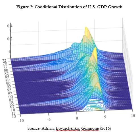
This evidence points towards deep linkages between macroeconomic and financial dynamics. Importantly, the empirical approach used to generate the conditional distributions is designed to capture nonlinear effects. The mean, variance, skewness and kurtosis of the conditional GDP distribution all depend significantly on financial conditions. In terms of magnitudes, movements in the first and second moment tend to be more important than movements in the third and fourth moments. Hence a conditionally Gaussian model where the conditional mean and the conditional variance of GDP depend on financial conditions performs well. This approach is used in the next Figure 3 to derive the conditional 5th and 95th quantile of GDP at the one year ahead horizon, clearly showing nonlinear dependence.
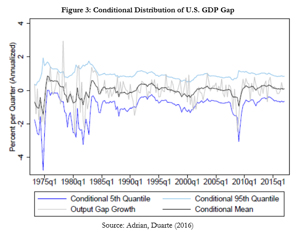
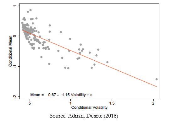
Another important observation that emerges is the negative dependence of the conditional GDP mean and the conditional GDP volatility, shown in Figure 4. When financial conditions deteriorate, the conditional mean declines and volatility increases, generating the negative relationship. For upper quantiles of the GDP distribution, movements in the mean and the volatility are more or less offsetting, resulting in the relatively stable right tail visible in Figures 2 and 3.
These findings suggest that the conditional distribution of GDP and financial conditions are tightly linked, and that the dependence appears to be nonlinear, i.e. the conditional variance of GDP and possibly higher moments depend significantly on financial conditions. Furthermore, risk to output is significantly linked to the financial cycle, i.e. the tendency of financial conditions to mean revert. And financial conditions are tightly linked to the term structure of interest rates, as we have seen in the regressions. The challenge lying ahead is to build parsimonious, tractable macrofinancial models that replicate these salient features, and that explain the term structure of interest rates.
A different approach
I will now turn to my approach to model these empirical facts within a tractable macrofinancial framework. The key challenge is to strike the balance between analytical tractability and richness of macrofinancial linkages in a meaningful way. This is based on recent joint work with Fernando Duarte (2016), who is at the New York Fed.
The starting point is a standard NK model that is augmented with a financial intermediary sector—call it the banking sector—that is subject to an occasionally binding Value-at-Risk (VaR) constraint. Hence, effective risk aversion is time varying as a function of the tightness of the VaR constraint. Importantly, we assume that the intermediary is also subject to preference shocks, which induce shifts in pricing of risk. Aggregate demand is pinned down by the intertemporal consumption-saving equation of the households, while aggregate supply is pinned down by a standard Phillips curve.
The model can be solved in closed form—with a pen and paper—but the solution is highly nonlinear. The interaction between real and financial dynamics is very rich by construction: intermediary preference shocks shift the pricing of risk via movements in the effective risk aversion of banks. Because of trading between banks and households (including through deposits), this tilts the IS-curve, impacting the output gap. The output gap in turn determines demand for goods. Given demand for goods, the Phillips curve determines inflation.
We also make a technical contribution, which brings us back to the term structure of interest rates. We derive the nonlinear equilibrium in closed form and then proceed by linearizing first and second moments separately. The rationale is that highly nonlinear dynamics are difficult to match empirically—any particular model of nonlinearity is probably misspecified. However, the evolution of first and second moments as a function of key state variables is the main driver of nonlinear evolution of macrofinancial linkages. Such state variables include the price of risk, the degree of intermediary leverage, the credit to GDP gap, etc. This approach is a very general one that can be applied to the range of macro-finance models that I mentioned earlier.
Within the context of our specific model, the VaR constraint induces a link between the conditional means and the conditional volatilities, producing feedback between financial premia (conditional volatilities) and expected levels of real macro variables (conditional means). When monetary policy in the context of sticky prices moves the real rate, that has two effects: it shifts the intertemporal savings decision in the Euler equation (the IS curve) as is standard in NK models, but it also acts on the tightness of the VaR constraint, thus moving the price of risk. Hence optimal monetary policy, which we derive analytically, conditions not just on the output gap and inflation, but also on the pricing of risk in the economy.
Both empirically, and in the model, macrofinancial linkages are derived from the observation that the conditional means and conditional volatilities both depend on the same set of state variables. The model generates the conditional GDP distribution that I plotted earlier: when financial conditions are easy, i.e. when the price of risk is compressed, the expected growth of GDP is high, while the conditional GDP volatility is low. Conversely, when financial conditions are tight, expected growth is low and conditional volatility is high. Hence for upper quantiles of GDP deteriorating financial conditions are relatively stable as the lower mean is offset by higher variance, whereas for lower quantiles, a lower mean and lower volatility are additive, leading to a more volatile left tail of the conditional distribution.
The model also features a volatility paradox. Periods of easy financial conditions are characterized by a buildup of financial intermediary leverage, making the financial system vulnerable to adverse shocks. When such shocks hit, intermediaries attempt to reduce their balance sheet size, pushing down asset prices, and increasing realized volatility. That leads to an endogenous tightening of the VaR constraint, which acts as an amplification mechanism for the initial and subsequent shocks. Hence a positive feedback loop turns into an adverse feedback loop eventually. Over time, on average, good times are followed by bad times, and hence the volatility paradox is generated in the model. The key driver of the financial cycle is the cycle in the pricing of risk, which corresponds to the cycle in the tightness of the intermediary funding constraint. Notably, these amplification mechanisms are present despite market completeness.
Monetary policy should take this intertemporal tradeoff into account. In our setup, optimal monetary policy is different than in the standard NK model: an optimal monetary policy rule should condition not only on the output gap and inflation but also on vulnerability. Furthermore, the presence of vulnerability breaks the divine coincidence of NK models: zero mean and zero volatility of the output gap are no longer simultaneously attainable. Of course, macroprudential policies can improve welfare further.
Macrofinancial dynamics and the term structure of interest rates
What does such an economy imply about term structure dynamics? The model that I sketched generates a nonlinear pricing kernel that matches the macro-financial linkages that I described. From the pricing kernel, we can simulate a term structure, and then study the properties of the term structure. In the short time that I have left, I will outline some preliminary results from this simulation exercise. The only shocks in the model are to financial intermediaries’ risk appetite, translating into shifts in the pricing of risk.
The simulation evidence from the model reproduces the earlier findings that the term structure of interest rates is only loosely related to macroeconomic variables, but is more closely related to financial conditions. The simulation is done within the macro-finance model of Adrian and Duarte (2016) that I described. Principal components are extracted from the simulated yields, and those PCs are then regressed on the output gap and inflation, and on the price of risk—the appropriate financial conditions index within the context of the model. While the underlying model has only one risk factor, the nonlinearity of equilibrium dynamics give rise to a multitude of significant principal components, as those are linear factors. Table 4 shows these regressions of the first three yield curve principal components on the macroeconomic factors and on financial conditions. Panel A shows the simulated economy using a standard Taylor rule, while Panel B shows the simulated economy using the optimal monetary policy rule that takes the economy’s vulnerability into account.
Table 4: Explaining Yield Curve Principal Components with Macroeconomic and Financial Variables using simulated data from Adrian and Duarte (2017)
Panel A: Monetary Policy that Ignores Financial Conditions
|
|
PC1 |
PC2 |
PC3 |
|
|
Inflation and output gap |
22% |
12% |
0% |
|
|
Financial conditions |
35% |
28% |
3% |
|
|
R-squared |
38% |
35% |
6% |
26% |
Panel B: Monetary Policy that Responds to Financial Conditions
|
|
PC1 |
PC2 |
PC3 |
|
|
Inflation and output gap |
26% |
4% |
0% |
|
|
Financial conditions |
35% |
39% |
13% |
|
|
R-squared |
41% |
41% |
13% |
32% |
Source: Inflation, the output gap, financial vulnerability and the yield curve PCs are computed from simulated data using the model in Adrian and Duarte (2017). The model is calibrated to reproduce Figure 3. Panel A uses Taylor rule coefficients of 1 for the output gap, 2 for inflation and zero for vulnerability. Panel B uses Taylor rule coefficients of 1 for the output gap, 2 for inflation and 2 for vulnerability.
The simulation results are remarkable. Even though the simulated model has only one risk factor, so that inflation, the output gap, and financial conditions are all functions of the same underlying factor, the magnitude of the R-squares are comparable to what we observe in the data. Furthermore, even though three principle components explain the vast majority of variation in the simulated yields, just as in the real data, they are only loosely related to macroeconomic variables. Finally, the optimal monetary policy rule that augments the classic Taylor rule by incorporating financial conditions beyond the output gap and inflation generates larger R-squares, as the degree of skewness of GDP is mitigated.
These results suggest that nonlinear macrofinancial dynamics might indeed be able to explain the following facts jointly in a parsimonious model:
- Macroeconomic and financial variables are driven by the same exact factors, but are related in a nonlinear fashion
- The term structure of interest rates is well described by a small number of yield factors
- The yield curve factors are only loosely related to macroeconomic variables
In our model, an affine term structure model would perform well, even though it is misspecified. A better approach would be a CIR type model that allows for conditional heteroscedasticity. In fact, by linearizing the conditional mean and conditional volatility of the model separately, we can produce a CIR type-pricing kernel. This approach is promising for future research on the intersection of macrofinancial modeling and the term structure of interest rates. The macro-finance model that I sketched has the potential to explain the three quantities that I showed at the beginning in a parsimonious fashion: the joint evolution of the natural real rate r*, the term premium, interest rate volatility, and the nominal yield curve.
To finish, let me briefly comment on the current macrofinancial environment. In the three largest advanced economies—the United States, Germany, and Japan—the unemployment rate is close to historical lows. Yet core inflation in those countries is below target. Hence the path of monetary tightening, i.e. the yield curve adjusted for term premia, is shallow, implying that the market perceives that interest rates will rise at only a very gradual pace. Estimates of r* are close to zero in all three regions. This suggests that the market is pricing in a low likelihood of recession in the near future, as reflected in the low observed market volatility. Of course, adverse shocks, or a resurgence of inflation might change that picture in the future, but markets currently give such adverse scenarios very low weight. Put differently, market pricing suggests a benign phase of the financial cycle. It is often during those benign times that financial vulnerabilities tend to build, hence monitoring financial stability is key: the IMF’s financial stability assessment of those risks will be provided in the upcoming Global Financial Stability Report in October.
Thanks for your attention. I am happy to take some questions.
References
Adrian, Tobias, Nina Boyarchenko, and Domenico Giannone (2016), “Vulnerable Growth,” Federal Reserve Bank of New York Staff Reports 794.
Adrian, Tobias, Richard K. Crump, and Emanuel Moench (2013), “Pricing the Term Structure with Linear Regressions,” Journal of Financial Economics, 110(1), 110-38.
Adrian, Tobias, Daniel M. Covitz, and J. Nellie Liang (2015), “Financial Stability Monitoring,” Annual Review of Financial Economics, 7, pp. 357-395.
Adrian, Tobias, Fernando Duarte (2016), “Financial Vulnerability and Monetary Policy,” Federal Reserve Bank of New York Staff Reports 804.
Adrian, Tobias, Daniel Stackman, and Erik Vogt (2016), “Global Price of Risk and Stabilization Policies,” Federal Reserve Bank of New York Staff Reports 786.
Brunnermeier, Markus K. and Yuliy Sannikov (2014), “A Macroeconomic Model with a Financial Sector,” American Economic Review, 104(2), 379-421.
Christensen, Ian and Ali Dib (2008), “The Financial Accelerator in an Estimated New Keynesian Model,” Review of Economic Dynamics, 11(1), 155-178.
Christiano, Lawrence J., Martin Eichenbaum, and Charles L. Evans (2005), “Nominal Rigidities and the Dynamic Effects of a Shock to Monetary Policy,” Journal of Political Economy, 113(1), 1-45.
Christiano, Lawrence J., Mathias Trabandt, and Karl Walentin (2011), “DSGE Models
for Monetary Policy Analysis,” In Benjamin M. Friedman, and Michael Woodford,
Handbook of Monetary Economics, Vol. 3A, pp. 285-367.
Clarida, Richard, Jordi Gali, and Mark Gertler (1999), “The Science of Monetary Policy: A New Keynesian Perspective,” Journal of Economic Literature, 37, 1661-1707.
Fernández-Villaverde, Jesus and Juan Rubio-Ramírez (2007), “Estimating Macroeconomic Models: A Likelihood Approach,” Review of Economic Studies, 74, 1059–1087.
Gali, Jordi and Tommaso Monacelli (2005), “Monetary Policy and Exchange Rate Volatility in a Small Open Economy,” Review of Economic Studies, 72, 707-734.
Gerali, Andrea, Stefano Neri, Luca Sessa, and Federico M. Signoretti (2010), “Credit and Banking in a DSGE Model of the Euro Area,” Journal of Money, Credit and Banking, 42(1), 107-141.
Gertler, Mark, Simon Gilchrist, and Fabio M. Natalucci (2007), “External Constraints on Monetary Policy and the Financial Accelerator,” Journal of Money, Credit and Banking, 39(2-3), 295-330.
Gertler, Mark and Peter Karadi (2011), “A Model of Unconventional Monetary Policy,” Journal of Monetary Economics, 58(1), 17-34.
Gertler, Mark and Nobuhiro Kiyotaki (2010), “Financial Intermediation and Credit Policy in Business Cycle Analysis,” in Benjamin M. Friedman and Michael Woodford, Handbook of Monetary Economics, 3A(11), 547-599.
Gurkaynak, Refet, Brian Sack, and Eric Swanson, (2005) “Do Actions Speak Louder Than Words? The Response of Asset Prices to Monetary Policy Actions and Statements,” International Journal of Central Banking, 1(1), 55-93.
Gurkaynak, Refet, Brian Sack, and Jonathan H. Wright, (2006) “The U.S. Treasury Yield Curve: 1961 to the Present,” Federal Reserve Board Finance and Economics Discussion Series 2006-28.
He, Zhiguo, and Arvind Krishnamurthy (2013) “Intermediary Asset Pricing” American Economic Review 103(2), 732-770.
Iacoviello, Matteo (2005) “House Prices, Borrowing Constraints, and Monetary Policy in the Business Cycle” American Economic Review 95(3), 739-764.
Kim, Don H., and Jonathan H. Wright (2005) “An Arbitrage-Free Three-Factor Term Structure Model and the Recent Behavior of Long-Term Yields and Distant-Horizon Forward Rates” Federal Reserve Board Finance and Economics Discussion Series 2005-33.
Laubach, Thomas, and John C. Williams (2003), “Measuring the Natural Rate of Interest,” Review of Economics and Statistics, 85(4), 1063-1070.
Obstfeld, Maurice, Kenneth Rogoff, Elhanan Helpman, and Effraim Sadka (2002) “Risk and Exchange Rates” Contemporary Economic Policy: Essays in Honor of Assaf Razin, Cambridge University Press.
Ranciere, Romain, Aaron Tornell, and Frank Westermann (2008) “Systemic Crises and Growth” Quarterly Journal of Economics 123(1), 359-406.
Rudebusch, Glenn D., and Tao Wu (2008) “A Macro‐Finance Model of the Term Structure, Monetary Policy and the Economy” Economic Journal 118(530), 906-926.
Rudebusch, Glenn D., and Eric T. Swanson (2012) “The Bond Premium in a DSGE Model with Long-run Real and Nominal” American Economic Journal: Macroeconomics 4(1), 105-143.
Schmidtt-Grohé, Stefanie and Martin Uribe (2003), “Closing Small Open Economy Models,” Journal of International Economics, 61, pp 163-185.
Smets, Frank and Raf Wouters (2007) “Shocks and Frictions in US Business Cycles: a Bayesian DSGE Approach” American Economic Review, 97(3), 586-606.
Woodford, Michael (2003) Interest and Prices: Foundations of a Theory of Monetary Policy, Princeton University Press.
[1] See also work by Fernandez-Villaverde and Rubio-Ramirez (2007) on model estimation, Gali and Monacelli (2005) as well as Schmidtt-Grohé and Uribe (2003) for open economy extensions, and Christiano, Trabandt, and Walentin (2011) for a discussion of the use of DSGE models in policy contexts.
[2] Researchers have been working on incorporating variation in the pricing of risk into otherwise standard macro models. A popular approach is to use the standard NK model, and to augment it with some variation in the pricing of risk. For example, Gerali et al. (2010), Iacoviello and Neri (2010), Gertler, Gilchrist, and Natalucci (2007), and Christensen and Dib (2008) have an otherwise standard NK model that allows for exogenous variation in risk premia at the longer end of the yield curve. Such models do generate a term structure, they are analytically tractable, and they speak to both macroeconomic and financial developments. But, the degree of macro-financial linkages is somewhat mechanical and the feedback between the real and the financial sector is nonexistent or limited. Obstfeld and Rogoff (2002) present an open economy framework that generates endogenous interest and exchange rate risk premia.
IMF Communications Department
MEDIA RELATIONS
PRESS OFFICER: Silvia Zucchini
Phone: +1 202 623-7100Email: MEDIA@IMF.org