Seven Questions About The Recent Oil Price Slump

IMF Blog, December 22, 2014

Source details

Canonical URL: Seven Questions About The Recent Oil Price Slump

Other formats

Bibliographic details

Authors: Rabah Arezki, Olivier Blanchard
Published: December 22, 2014

Executive summary

Oil prices have plunged, producing a net gain for world GDP between 0.3 and 0.7 percent in 2015 relative to a scenario without the drop in oil prices.
Both supply and demand factors contributed to the decline; supply factors appear to have played a dominant role.
Oil importers (advanced and emerging) generally benefit from higher household income, lower input costs, and improved external positions; oil exporters face lower revenues, fiscal and external pressure, and exchange rate challenges.
Financial stability risks have increased but remain limited to a handful of oil exporters so far; global linkages warrant vigilance.
Policy priorities: smooth fiscal adjustment in exporters, avoid abrupt fiscal cuts where possible, use the price decline to reform energy subsidies and taxes, and in the euro area and Japan use forward guidance to anchor medium-term inflation expectations.

Source: Rabah Arezki and Olivier Blanchard, December 22, 2014.

Causes of the price decline

Magnitude of decline:
- Oil prices have fallen by nearly 50 percent since June, 40 percent since September.
Relative movements:
- Metal prices have decreased substantially less than oil, suggesting oil-specific factors.
Demand vs supply:
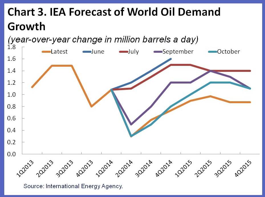
- Revisions of International Energy Agency demand forecasts and short-run supply elasticity imply unexpected lower demand can account for only 20 to 35 percent of the price decline.
- Supply-side contributors:
- Surprise increases in production, including faster Libyan recovery (September) and unaffected Iraqi production.
- Saudi Arabia’s announced intention not to counter rising supply and OPEC’s November decision to maintain a collective production ceiling of 30 million barrels a day.
- The shift by the swing producer changed expectations about future supply, pushing prices closer to competitive equilibrium (historical analogue: 1986 fall from $27 to $14 per barrel).
Financialization/speculation:
- Little evidence that financialization or speculation drove the decline; oil inventories reached their highest level in two years according to the International Energy Agency.

Persistence of the supply shift and future price paths

Key determinants of persistence:
- Whether OPEC/Saudi Arabia will cut production in the future (motives: sustain high price vs reduce non-OPEC profits/investment).
- How investment and oil production respond to low prices.
Investment signals:
- Rystad Energy: overall capital expenditure of major oil companies is 7 percent lower for the third quarter of 2014 compared to 2013.
- Rystad projections indicate capital expenditures will fall markedly through 2017.
Unconventional (U.S. shale) context:
- Unconventional oil accounts for 4 million out of a world supply of 93 million barrels a day.
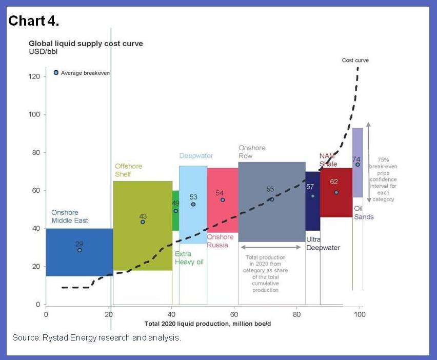
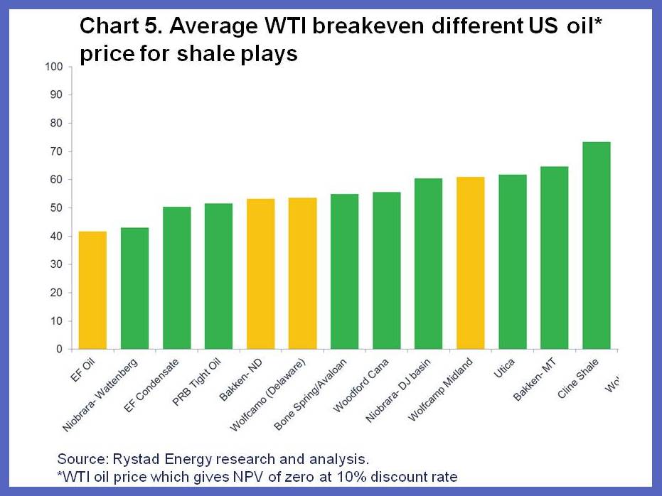
- Break-even prices for main U.S. shale fields (Bakken, Eagle Ford and Permian) are typically below $60 per barrel.
- At current prices (around $55 per barrel), Rystad projects production could decline moderately by about less than 4 percent in 2015; rates of return will be significantly lower.
Futures and uncertainty:
- Futures markets suggest partial recovery: expected recovery to $73 a barrel by 2019.
- Option-implied uncertainty (2019):
- 68% confidence band: $48 to $85.
- 95 percent band: $38 to $115.
Scenario detail (supply component timeline for Scenario 2):
- 2014: 60 percent
- 2015: 45 percent
- 2016: 30 percent
- 2017: 20 percent
- 2018: 10 percent
- 2019: zero

Global economic effects — simulations and quantitative results

Simulation framing:
- Two ceteris paribus simulations isolating the supply component of the price decline.
- Oil price path based on IMF price forecast (futures contracts).
- First simulation: supply shift accounts for 60 percent of the price decline and persists.
- Second simulation: supply shift starts at 60 percent but gradually goes to zero by 2019.
Global GDP effects (relative to baseline without the oil price drop):
- First simulation: increase in global output of 0.7 percent in 2015 and 0.8 percent in 2016.
- Second simulation: increase of 0.3 percent in 2015 and 0.4 percent in 2016.
Comparison with empirical estimates:
- Blanchard and Gali (2009): permanent 10 percent supply-driven oil price decrease raises U.S. output by about 0.2 percent.
- Given an approximate supply component of 25 percent (60% of a total decline of 40%), these imply an increase in output of about 0.5 percent.

Effects on oil importers

Transmission channels:
- Real income effect on consumption.
- Decrease in production costs leading to higher profits and investment.
- Effect on headline and core inflation and monetary policy response.
Cross-country variation:
- U.S. produces over half of the oil it consumes; real income effect smaller for the United States than for the euro zone or Japan.
- Energy intensity and oil cost share in GDP (average over 2004-2014):
- United States: 3.8 percent
- China: 5.4 percent
- India and Indonesia: 7.5 percent
Inflation pass-through assumption:
- Assumed pass-through of about 0.2; a decrease in core inflation of 0.2 percentage points when headline inflation decreases by 1 percentage point.
Simulated country impacts (two scenarios):
- China:
- 2015: GDP increases 0.4-0.7 percent above baseline.
- 2016: GDP increases 0.5-0.9 percent above baseline.
- United States:
- 2015: GDP increases 0.2-0.5 percent above baseline.
- 2016: GDP increases 0.3-0.6 percent above baseline.
Additional considerations not in simulations:
- Currency depreciations: yen and euro depreciated by 14 percent and 8 percent respectively since June, muting dollar-priced oil declines to 36 percent (yen) and 40 percent (euro).
- Energy taxes and specific tax structures: fixed per-unit energy taxes reduce consumer price declines when world prices fall.
- Subsidy reform: reducing energy subsidies will reduce the decline in consumer prices but free fiscal space for targeted transfers.
- Spillovers from exporters: low-income importers reliant on transfers (e.g., Petrocaribe), Caucasus and central Asia importers exposed to Russian slowdown, Mashreq countries and Pakistan exposed to declines in GCC transfers and remittances.

Effects on oil exporters

General effects:
- Real income and oil production profits decline.
- Fiscal deficits likely due to lower oil revenues.
Concentration and dependence examples:
- Russia: energy accounts for 25 percent of GDP, 70 percent of exports, and 50 percent of federal revenues.
- Gulf Cooperation Council (federal government revenue): oil accounts for 22.5 percent of GDP and 63.6 percent of exports.
- Africa:
- Gabon, Angola, Republic of Congo: oil exports account for 40-50 percent of GDP.
- Equatorial Guinea: oil exports account for 80 percent of GDP.
- Angola, Republic of Congo, Equatorial Guinea: oil accounts for 75 percent of government revenues.
- Latin America:
- Ecuador and Venezuela: oil contributes about 30 percent and 46.6 percent to public sector revenues, and about 55 percent and 94 percent of exports respectively.
Fiscal break-even and budget vulnerability:
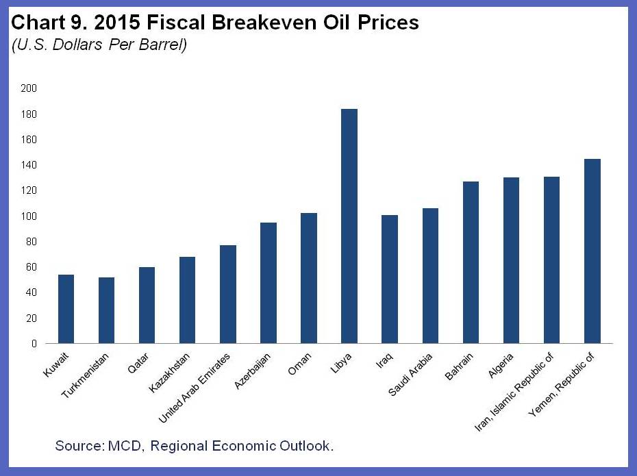
- Fiscal break-even prices vary and are often very high:
- Kuwait: $54 per barrel
- Libya: $184 per barrel
- Saudi Arabia: $106 per barrel
- Budgetary oil prices:
- Ecuador: $79.7
- Venezuela: $60
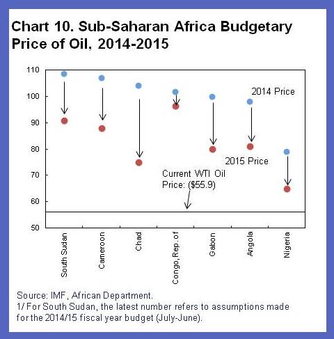
- For many African countries, budgetary oil prices were revised down for 2015.
Policy capacity and mitigation:
- Some countries have fiscal rules and saving funds (e.g., Norway) to cushion adjustment.
- Others face fiscal tightening, lower output, and depreciation pressure; fixed exchange rate regimes complicate adjustment.
- Where inflation expectations are not well anchored, depreciation may induce higher inflation.

Financial implications

Direct and indirect channels:
- Lower oil prices weaken energy firms’ finances and banks with exposure to the energy sector.
- Exchange rate adjustments amplify balance sheet risks for dollar-denominated debtors.
Indicators of stress:
- Proportion of energy firms with interest coverage ratio below 2: 31 percent in emerging countries.
- CEMBI spreads have increased by 100 basis points since June.
Banking sector resilience:
- Past stress tests found only a few banks in some oil exporters would need recapitalization of a few points of GDP; current buffers and profitability have changed since those tests.
- Russia: rapidly evolving financial conditions due to sanctions and currency movements.
Currency movements:
- Russian rouble depreciation: 40 percent so far this year, and 56 percent since September.
- Depreciations help adjustment but exacerbate dollar-denominated debt burdens and may lead to high inflation if expectations are unanchored.
Global banking exposure and tail risk:
- Global banking system exposure to oil exporters is unlikely to cause more than a moderate increase in provisioning, partially offset by improving credit in oil importers.
- Tail risk remains: large price and exchange rate moves can raise global risk aversion, repricing risk and shifting capital flows (interaction with events in Russia highlighted).

Policy recommendations

Common and cross-cutting:
- Use the fall in oil prices as an opportunity to reduce energy subsidies and redirect savings to targeted transfers.
- Consider increasing energy taxes in some advanced economies and use revenue to lower distortionary taxes (e.g., labor taxes).
For oil importers:
- In normal macro conditions: monetary policy should keep inflation expectations anchored and stabilize core inflation; exchange rate appreciation from improved current accounts is natural and desirable.
- In current context (output gaps, inflation below target, zero lower bound):
- Demand boost from lower oil prices is welcome.
- Forward guidance is crucial in the euro area and Japan to anchor medium-run inflation expectations and avoid sustained deflation.
For oil exporters:
- Where fiscal space exists (savings funds, fiscal rules): allow larger deficits temporarily and draw on funds to smooth adjustment, especially under fixed exchange rates.
- Where fiscal space is limited: pursue fiscal consolidation, allow larger real depreciation, and maintain strong monetary frameworks to prevent depreciation-induced inflationary spirals.
- Avoid abrupt curtailment of fiscal spending where possible; prioritize smoothing to limit output and financial stress.

Source: IMF blog post "Seven Questions About The Recent Oil Price Slump" (Rabah Arezki and Olivier Blanchard, December 22, 2014).

References

- https://www.imf.org/wp-content/uploads/2014/12/oil-2.jpg
- https://www.imf.org/wp-content/uploads/2014/12/oil-3.jpg
- https://www.imf.org/wp-content/uploads/2014/12/oil-4.jpg
- https://www.imf.org/wp-content/uploads/2014/12/oil-5.jpg
- https://www.imf.org/wp-content/uploads/2014/12/oil-6.jpg
- https://www.imf.org/wp-content/uploads/2014/12/oil-9.jpg
- https://www.imf.org/wp-content/uploads/2014/12/oil-10.jpg