Speech

Alternative Monetary Policy Paths and Downside Risk

October 29, 2018

Economic forecasts usually provide point estimates for the conditional mean of GDP growth (or the GDP gap). However, such point forecasts ignore risks around the central forecast and, at times, may paint an overly optimistic picture of the state of the economy. In fact, policy makers' focus on risks around the forecast has increased in recent years. In Europe, the Governing Council of the ECB commonly discusses the balance of risks to growth and inflation, as does the Federal Open Market Committee in the United States. At the same time, surveys of economists, market participants and professional forecasters all collect respondents’ beliefs regarding the probability distribution around the point forecast. ^[1]

Of course, there is an econometric literature on density forecasting. Economists long argued that policy makers would surely want to know the whole conditional distribution of the relevant state variables to take optimal policy decisions (Timmermann 2000). ^[2] But this literature has had little practical impact on monetary policymaking as the econometrics of density forecasting is rather technical.

Furthermore, the monetary policy literature has not, to date, come up with structural models that capture the conditional density of relevant state variables in a parsimonious yet policy-relevant fashion. The literature tends to focus on linearized models with either constant volatility, which does not generate meaningful conditional densities, or where volatility varies exogenously over time. ^[3]

When central banks produce forecast distributions, those are usually computed either via resampling procedures of linear models, or via purely judgmental approaches whereby likelihoods over alternative scenarios are combined. The challenge with resampled distributions is that they are not conditional on the state of the economy. While judgment is very important in policymaking, translating views about alternative scenarios to generate forecast distributions is challenging in practice. ^[4]

In this speech, I will argue that it is time for practical monetary policymaking to start incorporating endogenous forecast distributions. This is due to three advances in modeling and estimation:

· First, density forecasting has become relatively straightforward to implement (Adrian, Boyarchenko, Giannone 2018). Financial conditions have been found to be powerful forecasting variables for the whole future GDP distribution. Financial vulnerability manifests as downside risk to output (gap or growth).

· Second, I will sketch a parsimonious New Keynesian model with financial vulnerability that matches closely those forecast densities (Adrian and Duarte 2018). The model generates conditional forecasts of the whole distribution and allows for closed form expressions of the optimal policy rule as a function of financial vulnerability.

· Third, I will argue that the monetary policy process should take the endogenous evolution of risk into account in considering alternative policy paths, in addition to the impact of policy on inflation and the output gap.

Conditional Density Forecasting of Output and Inflation

Adrian, Boyarchenko, Giannone (2018) propose a parsimonious two step estimator for forecasting densities of output:

· First, regress future output (growth or gap) on current output and current financial conditions using quantile regressions. In quantile regressions, instead of estimating a conditional mean, the conditional quantile is assessed, thus allowing estimation of the whole conditional distribution. (Economic conditions are additional regressors.)

· Second, fit a flexible distribution function across quantiles at every point in time, thus generating a conditional time series of output densities.

The estimators have excellent out of sample performance relative to naïve random walk estimators, more complicated Bayesian approaches, or fully parametric maximum likelihood approaches. While in practice many alternative approaches can be used, this estimation method is particularly robust and straightforward to implement.

Figure 1: One Year Ahead Conditional GDP Growth, 1973-2016

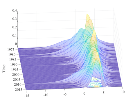
From Adrian Boyarchenko Giannone (2018)

Adrian, Boyarchenko, Giannone (2018) uncover the following stylized facts:

1) The conditional volatility of future GDP is predicted primarily by financial conditions.

2) The one quarter and one year ahead conditional density of GDP is primarily evolving as a function of how the conditional mean and the conditional volatility change over time, while higher moments such as conditional skewness and kurtosis only varying slightly.

3) The conditional mean and conditional volatility are negatively correlated, which gives rise to an unconditional GDP distribution that is strongly skewed to the left. This can be seen in Figure 1.

Further work is expanding on these results by studying the term structure of downside risk to GDP growth (Adrian, Grinberg, Liang, Malik 2018). Growth-at-risk is measured by the (lower) 5th percentile of future GDP growth conditional on financial conditions. The shape of the estimated growth-at-risk term structure is consistent with endogenous risk-taking and the volatility paradox. Periods of easy financial conditions are characterized in the short run by low downside risks and high expected growth, but there is a reversal in the medium term as easy financial conditions forecast a large increase in downside risks. Conversely, in times of recessions or crises when financial conditions are particularly tight, downside risks in the near-term are large, but diminish in the medium-term.

Figure 2: Term Structure of Growth at Risk by FCI, 2018
(Projected 5^th percentile of GDP growth, in percent)

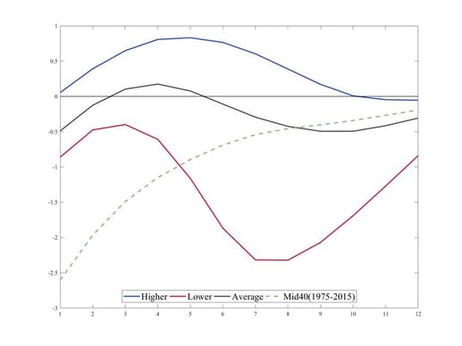
Updated from Adrian Grinberg Liang Malik (2018)

The current estimate of the term structure of Growth-at-Risk across 11 advanced economies is shown in Figure 2 (based on updated data from Adrian, Grinberg, Liang, Malik 2018). The prevailing easier-than-average financial conditions across countries help limit downside risks to growth in the near term relative to mid-range financial conditions over the past 40 years. But today’s easier conditions also suggest larger downside risks two years from now, and as soon as in one year if the economy is also currently in a credit boom. Shifts in financial conditions due to monetary policy actions and other factors thus can differentially impact short and medium term downside risks to growth, creating a potential intertemporal risk tradeoff for policy makers.

A New Keynesian Model with Financial Vulnerability

Since the seminal contributions of Bernanke, Gertler, Gilchrist (1999) (BGG) and Kiyotaki, Moore (1997), monetary economists have been working on models that incorporate financial frictions in applied monetary policy models. A huge effort is underway to develop methods to solve such models globally, or up to high order, as they are generically nonlinear. ^[5] In practice, such highly nonlinear models have not proven relevant for policy purposes, as the exact nature of the nonlinearity is highly model specific, and difficult to fit to the data. Instead, macro-financial models that are widely used in central banks today rely predominantly on first order solution methods, and model financial frictions up to first order. ^[6]

I would like to argue here that the way forward might be somewhat simpler: Instead of considering fully nonlinear models, I would like to propose that models with endogenous second moments, i.e. volatilities of output (or, more precisely, of the output gap) as a function of state variables might be sufficiently rich as the source of nonlinearity. In the type of model that I have in mind, the reduced form is very closely related to standard first order models, but the error terms feature endogenous volatilities that depend on state variables in a theory consistent fashion.

Figure 3: Conditional GDP Gap Mean and Variance

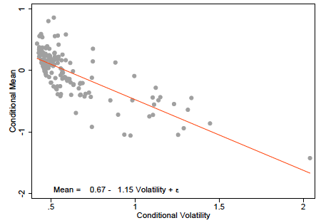
From Adrian Duarte (2018)

In fact, while the setup that I propose shares many features with the textbook New Keynesian (NK) model (Woodford 2003, Gali 2008), it is not linear and so doesn’t suffer from “certainty equivalence”. In other words, in the model risk matters and conditional second moments are not restricted to be constant. That restriction turns out to be strongly rejected in the data: conditional first and second moments are tightly linked and, importantly, the conditional mean and conditional volatility are negatively related as shown in Figure 3.

Adrian and Duarte (2018) solve a micro founded New Keynesian model with financial vulnerability in a fully nonlinear fashion, and then study the reduced form of the model. We will refer to that model by NKV (New Keynesian Vulnerability) model, in contrast to the standard NK model. The reduced form NKV model is a standard NK model with endogenous second moments that are linear functions of the state variables.

The NKV model allows for an analytical solution to the optimal policy rule. During booms, when the output gap is closed or positive and inflation is at or above target, the optimal rule is slightly tighter than the standard Taylor rule, thus leaning slightly against the buildup of financial vulnerabilities during times of easy financial conditions. ^[7] Furthermore, during times of a large output gap, monetary policy is looser than under a standard Taylor rule. That is, monetary policy in the recovery phase is easier than the standard Taylor rule in order to induce risk taking, which helps to more quickly close the output gap.

In follow-up work, the model is calibrated to 21 economies (both advanced and emerging), and estimations show that the welfare gains from using the optimal policy rule can be sizable (Adrian, Duarte, Grinberg, Mancini-Griffoli, 2017). Importantly, these welfare gains are not achieved because the central bank pursues a financial stability objective. Instead, the central bank is assumed to have an inflation-targeting mandate, but the resulting optimal monetary policy rule is a flexible inflation-targeting rule that conditions on financial vulnerability. ^[8]

Alternative Policy Paths with Endogenous Risk

Adrian, Duarte, Liang, Zabczyk (2018) build upon this work (Adrian and Duarte) by studying the properties of a reduced form NKV model with endogenous risk in discrete time. This model is exactly like the standard NK textbook three equation model, with two exceptions. First, it features financial vulnerability as an additional state variable, and hence the model has four equations. Second, there are two new parameters. One parameter determines the slope of the conditional output volatility (which is measured by financial conditions) as a function of the expected output gap. This slope corresponds to the risk return-tradeoff discussed earlier. The magnitude of the slope determines the “vulnerability channel”, as it pins down how vulnerability depends on expected growth. The second parameter governs the degree to which expected growth depends on the pricing of risk, and thus appears in the IS curve. This second channel is the “financial accelerator” of BGG. Hence in a very parsimonious model, we not only capture the “vulnerability channel”, but also the “financial accelerator channel”. These new parameters are fully micro founded in Adrian and Duarte (2018), though other micro foundations could surely be used.

Now, let me turn to an important third point I want to make this evening. I would like to argue that the merits of alternative policy paths in monetary policy decision-making should be analyzed in setups such as the NKV, which account for endogenous conditional risk and thus more fully capture the challenging tradeoffs facing policymakers. In particular, when comparing alternative rules, monetary policy makers should not only consider the paths of inflation and output, but also the endogenous path of output vulnerability (which maps into financial conditions in the NKV model). I will illustrate this point by comparing the optimal rule of the NKV model that takes financial vulnerability into account to the standard 1993 Taylor rule. ^[9]

Figure 4: Alternative Policy Paths for Output, Inflation, and Vulnerability

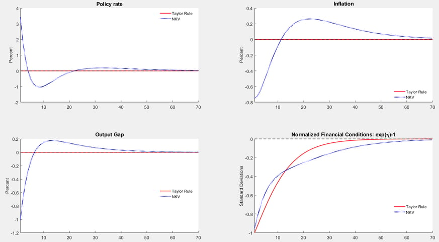
From Adrian, Duarte, Liang, Zabczyk (2018), preliminary

This Figure 4 is the one I want you to take home tonight. It shows the policy path and economy with an NKV rule—a Taylor rule with the addition of financial conditions—relative to the standard Taylor rule. The model is calibrated to start where inflation is roughly at target and the output gap is closed. Hence the usual inflation-real activity tradeoff does not come into play. But financial conditions are calibrated as very loose to start, and a NKV rule would prescribe a policy tightening to tighten financial conditions and increase output volatility more sharply in the near term than under a Taylor rule (which ignores financial conditions). Once financial conditions become less loose, monetary policy becomes less restrictive, and the output and inflation gaps close.

The crossing of the lines showing the path of financial conditions shows the benefit of the NKV rule relative to the Taylor rule. Under the Taylor rule, financial conditions are tighter and thus conditional output volatility is greater than under the NKV rule in the medium term. This illustrates the intertemporal risk tradeoff, where higher conditional volatility in the near-term may yield benefits in the form of lower volatility over the medium-term.

The model is symmetric. When the output and inflation gaps are closed, and financial conditions are relatively tight, the NKV rule would prescribe looser monetary policy than the Taylor rule, in order to increase risk taking in the short term.

Of course, what the “right decision” is for the policy maker depends on his or her preferences, including the discount factor, risk aversion, and the intertemporal elasticity of substitution. In an actual monetary policy setting, any decision would require policymakers’ judgment given lack of precision in measuring the output and inflation gaps in real time, and one might want to use a more realistic medium-sized DSGE model that fits the data along various additional dimensions. Moreover, any outcome will also reflect the ability of the policy maker to communicate clearly its objectives, how to measure them and over what time periods.

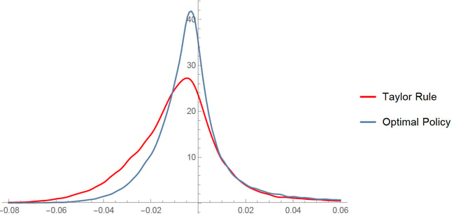
The key takeaway is that the policy maker who is aware of and tries to actively mitigate vulnerability, in addition to the usual focus on inflation gap and the output gap, will reduce negative skewness of the output gap over time, as is illustrated in Figure 5. In other words, prudent monetary policy in the presence of endogenous risk mitigates downside risks to GDP. We can surely all agree that this is a desirable outcome.

Figure 5: Steady State Output Gaps under the NKV and the Taylor Rule

From Adrian and Duarte (2018)

Macroprudential Policy

The overall safety and soundness of the financial system has to be addressed via structural prudential tools, both micro- and macroprudential. Those determine the overall resilience of the economy to shocks. The subject of the speech has been cyclical risk, and how it impacts monetary policy in practice.

The use of cyclical macroprudential tools can mitigate downside risks to GDP. Hence the NKV framework can be used to model monetary and cyclical macroprudential policies jointly. Macroprudential policy is unlikely to ever take care of downside risks entirely, as macroprudential tools and governance have limitations, and pronounced cyclical variation in downside risks persists. Hence in practice monetary policy does track downside risks.

Tracking risks to the forecast is very much in the spirit of the conduct of monetary policy today where monetary policy committees receive regular financial stability briefings and regularly consider the balance of risks. References to risks by monetary policy makers have been increasing in recent years, and some appear to react to shifts in financial conditions.

Furthermore, macroprudential tools usually take several quarters, and some cases a year or more, to be phased in, and the impact on economic activity might be even less timely. In contrast, monetary policy decisions are implemented immediately.

Conclusion

Let me conclude. I have argued here tonight that models of optimal monetary policy should take into account the endogeneity of risk, in three steps:

1) Data strongly suggests that the conditional volatility of output depends on financial conditions, and gives rise to an intertemporal risk-return tradeoff for policy makers. This finding holds across countries and across time.

2) Endogenous risk can be parsimoniously modeled in an NKV model with risk as an additional endogenous state variable, and with only two additional parameters relative to the standard NK model, one that governs the “financial vulnerability,” the other that governs the “financial accelerator.” Such a model is analytically tractable and captures the stylized facts described earlier.

3) This framework can provide the policy maker with an endogenous forecast distribution. The NKV model generates highly skewed and fat-tailed unconditional output distributions, even when shocks are Gaussian. In considering alternative policy paths, I have argued that policy makers should also consider the future path of risk.

With that, I would be happy to answer your questions.

Literature

Adrian, Tobias, Nina Boyarchenko, and Domenico Giannone (2018) “ Vulnerable Growth ” American Economic Review, forthcoming.

Adrian, Tobias and Fernando Duarte (2018) “ Financial Vulnerability and Monetary Policy ” Federal Reserve Bank of New York Staff Reports 804, December 2016.

Adrian, Tobias, Fernando Duarte, Nellie Liang, Pawel Zabczyk (2018) “Monetary Policy with Endogenous Risk” work in progress.

Adrian, Tobias, Fernando Duarte, Federico Grinberg, Tommaso Mancini-Griffoli (2017) “ Monetary Policy and Financial Conditions: A Cross-Country Study ” In: Advancing the Frontiers of Monetary Policy, International Monetary Fund, edited by Adrian, Laxton, Obstfeld, pp. 83-106.

Adrian, Tobias, Federico Grinberg, Nellie Liang and Sheheryar Malik (2018) “ The Term Structure of Growth at Risk ” International Monetary Fund Working Paper 18/180

Adrian, Tobias, Nellie Liang (2018) “ Monetary Policy, Financial Conditions, and Financial Stability ” International Journal of Central Banking 14(1), pp. 73-131.

Alessi, Lucia, Eric Ghysels, Luca Onorante, Richard Peach, and Simon Potter (2014) “Central Bank Macroeconomic Forecasting during the Global Financial Crisis: the European Central Bank and Federal Reserve Bank of New York Experiences” Journal of Business & Economic Statistics 32(4), pp. 483-500.

Andreasen, Martin, Jesús Fernández-Villaverde, and Juan Rubio-Ramírez (2016) “The Pruned State-Space System for Non-Linear DSGE Models: Theory and Empirical Applications” working paper.

Bernanke, Ben S., Mark Gertler, Simon Gilchrist (1999) “The Financial Accelerator in a Quantitative Business Cycle Framework” Handbook of Macroeconomics 1, pp. 1341-1393.

Cai, Michael, Marco Del Negro, Marc Giannoni, Abhi Gupta, Pearl Li, and Erica Moszkowski (2018) “DSGE Forecasts of the Lost Recovery” Federal Reserve Bank of New York Staff Report 844.

Dou, Winston, Andrew Lo, Ameya Muley, and Harald Uhlig (2018) “Macroeconomic Models for Monetary Policy: A Critical Review from a Finance Perspective” Working Paper.

Fernández-Villaverde, Jesús, Pablo Guerrón-Quintana, and Juan Rubio-Ramírez (2015) “Estimating Dynamic Equilibrium Models with Stochastic Volatility” Journal of Econometrics 185(1), pp. 216-229.

Galí, Jordi (2008) Monetary Policy, Inflation, and the Business Cycle: An Introduction to the New Keynesian Framework , Princeton University Press.

Justiniano, Alejandro and Giorgio E. Primiceri (2008) “The Time-Varying Volatility of Macroeconomic Fluctuations” American Economic Review , 98(3):604-41.

Kiyotaki, Nobuhiro, and John Moore (1997) “Credit Cycles” Journal of Political Economy 105(2), pp. 211-248.

Manganelli, Simone and Lutz Kilian (2008) “The Central Banker as a Risk Manager: Estimating the Federal Reserve´s Preferences Under Greenspan” Journal of Money, Credit, and Banking 40, pp. 1103-1129.

Sims, Christopher A., and Tao Zha (2006) “Were there Regime Switches in U.S. Monetary Policy?” American Economic Review, 96(1): 54-81.

Svensson, Lars EO (1997) “Inflation Forecast Targeting: Implementing and Monitoring Inflation Targets” European Economic Review 41(6), pp. 1111-1146.

Taylor, John B. (1993) “Discretion versus Policy Rules in Practice” In: Carnegie-Rochester Conference Series on Public Policy 39, pp. 195-214).

Timmermann, Allan (2000) “Density Forecasting in Economics and Finance” Journal of Forecasting 19(4), pp. 231-234.

Woodford, Michael (2003) Interest and Prices: Foundations of a Theory of Monetary Policy, Princeton University Press.

Endnotes